欢迎来到本博客
>
博主优势: 博客内容尽量做到思维缜密,逻辑清晰,为了方便读者。
>
座右铭:行百里者,半于九十。

摘要
本研究开发了两种新颖的算法:准对立气味代理优化(QOBL-SAO)及其莱维飞行变体(LFQOBL-SAO),并将它们的性能与传统的气味代理优化(SAO)进行了比较。进行了两项研究。首先,在解决十个基准函数和五个CEC2020真实世界优化问题方面,测试了这些新颖算法的能力。其次,将它们应用于为尼日利亚村庄的一家医疗中心优化混合光伏(PV)/风力/电池、PV/电池和风力/电池电力系统。使用上述位置的负载需求、光伏和风力概况开发了混合系统。所有仿真均在MATLAB软件中进行。结果表明,这些新颖算法能够解决基准函数和CEC2020真实世界约束优化竞赛。特别是,QOBL和LF-QOBL的性能与IUDE、MAgES和iLSHAD算法等表现最佳的函数一样出色。然而,在收敛时间、最低能量成本(LCE)和总年化成本(TAC)方面,这些新颖算法在光伏/风力/电池优化应用中优于SAO。采用LFQOBL-SAO和QOBL-SAO时,混合光伏/风力/电池系统是成本效益最高的,其TAC值为15100美元。此外,结果表明LFQOBL-SAO方法准确且优于QOBL-SAO和SAO算法。
介绍
温室气体(GHG)排放引起了这一代人的关注,由于技术进步、人口增长以及全球变暖现象的令人信服的证据,人们越来越专注于利用可再生能源(RES)[1],[2]。在公共事业网络不可用的孤立和偏远地区,RES被确定为可行的电力供应解决方案[3],[4]。RES包括风能、太阳能、生物质能、地热能以及其他自然资源。这些能源被认为是最丰富的,因为它们几乎可以在地球的任何地方找到,而且可能永远不会耗尽,但它们也是最不可预测的[5],[6]。与化石燃料相比,大多数RES是间歇性的,并受天气影响,对能源生产产生负面影响。为了解决这个问题,RES可以与其他常规能源和能量存储系统结合,提供更可靠的能源来源。系统内负载需求的突然增加也可以通过将这些RES以混合形式结合来满足[7],[8]。
部分代码:
clc;close all;
format long
tic
Data=xlsread('Val_Data.xlsx');
N=250;%input('Provide the Number of Smell Molecules:=');%INITIAL POPULATION
clc
T=3;%Temperature of gas molecules.
% fitness=input('Press 1 to Select Ackley[D=2]\
Press 2 to Select Adjiman[D=2]\
Press 3 to Select Alpin F1[D=2]\
Press 4 to Select Beale[D=2]\
Press 5 to Select Bird[D=2]\
Press 6 to Select Bohachevsky[D=2]\
Press 7 to Select Boot[D=2]\
Press 8 to Select Box[D=3]\
Press 9 to Select Bukin F6[D=2]\
Press 10 to Select Colville[D=4]\
Press 11 to Select CM[D=2]\
Press 12 to Select Cross-in-Tray[D=2]\
Press 13 to Select Dejong F4[D=2]\
Press 14 to Select Easom[D=2]\
Press 15 to Select Egg Crate[D=2]\
Press 16 to Select Ellipsoid[D=30]\
Press 17 to Select Goldstein Price[D=2]\
Press 18 to Select Grienwank[D=30]\
Press 19 to Select Holder Table 1[D=2]\
Press 20 to Select Kowalik[D=4]\
Press 21 to Select LM F1[D=2]\
Press 22 to Select Michalewicz[D=5]\
Press 23 to Select Matyas[D=2]\
Press 24 to Select Mishra[D=30]\
Press 25 to Select McComic[D=3]\
Press 26 to Select Neumaier F3[D=2]\
Press 27 to Select Quadratic[D=30]\
Press 28 to Select Rastrigin[D=5]\
Press 29 to Select Rosenbrock[D=2]\
Press 30 to Select Sphere[D=30]\
Press 31 to Select Styblinkis Tang[D=2]\
Press 32 to Select Step[D=5]\
Press 33 to Select Sal[D=30]\
Press 34 to Select Schaffer[D=2]\
Press 35 to Select Shchwefel[D=2]\
Press 36 to Select Subert F1[D=5]\
Press 37 to Select Watson[D=6]\
Press 38 to Select Yang F3[D=2]\
Press 39 to Select Zirilli[D=2]\=');
% itr=300;%input('Provide the value of iteration:=');
D=3;%input('Provide the Search Dimension:=');%Number of decision variables or problem dimension.
K=1.38064852*10^(-23);% This is the boltzman constant
Iter=100;
Run=50;
SN=2.5;
lb=[0,0,0];%Lower Bound of Decision Variables
ub=[100,100,50];%Upper bound of decision variables
m=2.4;%This is the mass of the molecules.
% Initial population (position) of the gas molecules as follows
tic
CostFunction=@AnualCost;
for R=1:Run
for k=1:Iter
for i=1:N
for j=1:D
molecules(i,j)=lb(j)+rand()*(ub(j)-lb(j));%Defind the initial positions of the smell molecules.
end
end
% molecules=rand(N,D);
v=molecules*0.1;
molecules=molecules+v;%Initial populaation of SAO
molecules=Quasi_Oppositional(molecules,lb,ub);
for i=1:N
y(i)=CostFunction(molecules(i,:));%Evaluate the fitness of the initial smell molecules
end
[ymin,index]=min(y);%Obtain the fitness of the best molecule
x_agent=molecules(index,:);%Determin the agent
olf=3.5;%ymin/(sum(y)/N);%Determine the Olfaction capacity of the agent.
% iteration=0;
% while iteration<=itr
% Implementing the sniffing mode
for i=1:N
for j=1:D
% Update the molecular Velocity
v(i,j)=(v(i,j)+rand*sqrt(3*K*T/m));
end
end
% perform sniffing
for i=1:N
for j=1:D
molecules(i,j)=molecules(i,j)+v(i,j);
end
end
for i=1:N
ys(i)=CostFunction(molecules(i,:));
end
[ysmin,sindex]=min(ys);
xs_agent=molecules(sindex,:);
[ysmax,sidx]=max(y);
x_worst=molecules(sidx,:);%Determin the position of worst smell molecule
if ysmin<ymin
xs_agent=molecules(sindex,:);
ymin=ysmin;
end
%%
%Evaluate the Trailing mode
for i=1:N
for j=i:D
molecules(i,j)=molecules(i,j)+rand*olf*(x_agent(1,j)-abs(molecules(i,j)))...
-rand*olf*(x_worst(1,j)-abs(molecules(i,j)));
end
end
%Make sure no smell molecules excape the boundary
for i=1:N
for j=1:D
if molecules(i,j)<lb(j)
molecules(i,j)=lb(j);
elseif molecules(i,j)>ub(j)
molecules(i,j)=ub(j);
end
end
end
%Evaluate the fitness of the Trailing mode
for i=1:N
yt(i)=CostFunction(molecules(i,:));
end
[ytmin,tindex]=min(yt);
%%
% Compare the fitness of the trailing mode and the sniffing mode
% and implement the random mode
for i=1:N
for j=1:D
if yt(i) < ys(i)
Best_Molecule(i,j)=yt(1,1);
elseif yt(i) > ys(i)
molecules(i,j)=molecules(i,j)+rand()*SN;
molecules(i,j)=molecules(i,j)+(v(i,j)+rand*sqrt(3*K*T/m));
molecules(i,j)=molecules(i,j)+rand*olf*(x_agent(1,j)-abs(molecules(i,j)))...
-rand*olf*(x_worst(1,j)-abs(molecules(i,j)));
end
end
end
molecules=Quasi_Oppositional(molecules,lb,ub);
for i=1:N
ybest(i)=CostFunction(molecules(i,:));
end
[SmellObject,Position]=min(abs(ybest));
% W=molecules(Position)
% if iteration==1
% disp(sprintf('Iteration Best particle Objective fun'));
% end
% disp(sprintf('%8g %8g %8.4f',iteration,Position,SmellObject));
Object(k)=sort(SmellObject,'descend');
% disp(['Iteration ' num2str(k) ': Smell Object=' num2str(Object(k))]);
% iteration=iteration+1;
% end
end
% disp('The Smell Object is Obtained as: ');
Best_Object=sort(Object,'descend')';
% Best_Object=Object;
% disp('The Object Evapourating the Smell is')
[Smell_Object,Pos]=min(Object);
BestCost_Run(R)=Smell_Object;
end
toc
% Y=molecules(Position)
smell=round(molecules(Pos,:));
Pconv=375.62;%2000;% Converter/Inverter Price
Npv=smell(:,2)
Nwt=smell(:,1)
Nbat=smell(:,3)
Nconv=3;
Speed=Data(:,2);
Ins=Data(:,1);
% disp('The Power of PV System is: ')
CRF=0.070952457299230;
Ppv=PvPower(Ins)';
Pwt=WindPower(Speed)';
E_Load=Data(:,3);
Pl=E_Load;
Cwt=144.3;%1250;% Unit Cost of Wind Turbine
Cpv=31.2;% 240 Unit Cost of PV Pannels
%(Npv*Ppv)+(Nwt*Pwt)>=E_Load
E_Gen=(Npv*Ppv)+(Nwt*Pwt);
%%
DOD=0.8;% Battery depth of discharge
Sbat=2.4;%Battery norminal capacity
Cmain_wt=154.3;% Maintanace cost of wind turbine
Cmain_pv=800;% Maintanace cost of PV Pannels
% Cmain_bat=90.95;% Maintanace cost of bat Pannels
Cbat=90.95;
Ccon=InverterWorth(Pconv,j);
SOCmax=2.4;
SOCCmin=(1-DOD)*Sbat;
SOCC1=abs(SOCC(Ppv,Pwt,Pl))';
SOCCmin<=SOCC1<=SOCmax;
SOCD1=abs(SOCD(Ppv,Pwt,Pl));
SOCDmin=SOCCmin;
if E_Gen<E_Load
SOC=SOCD(Ppv,Pwt,Pl)';
else
SOC=abs(SOCC(Ppv,Pwt,E_Load))';
end
PvCost=CRF*Cpv*Npv+(Cmain_pv*Npv)
CwtCost=CRF*Nwt*Cwt+(Cmain_wt*Nwt)
ConvCost=Nconv*InverterWorth(Pconv,j);
Bat_Cost=CRF*Nbat*Cbat
Conv_Cost=CRF*Nconv*Ccon
Total_Cost=PvCost+CwtCost+ConvCost+Conv_Cost+Bat_Cost
% Total_Cost=Smell_Object
Excess=Total_Cost-Smell_Object;
% Total_Cost=Smell_Object
LCE=(sum(E_Gen))/(Total_Cost+Smell_Object)
LPSs=LPS(Pl,Ppv*Npv,Pwt*Nwt,SOC);
LPSP=abs(LPSs/sum(Pl))';
disp('Loss of Power Supply Probability is: ')
LPSP=mean(mean(LPSP))*10^-3
disp('')
disp('')
disp('########The Excess Energy:######## ')
E_Ex=mean(E_Gen-E_Load)
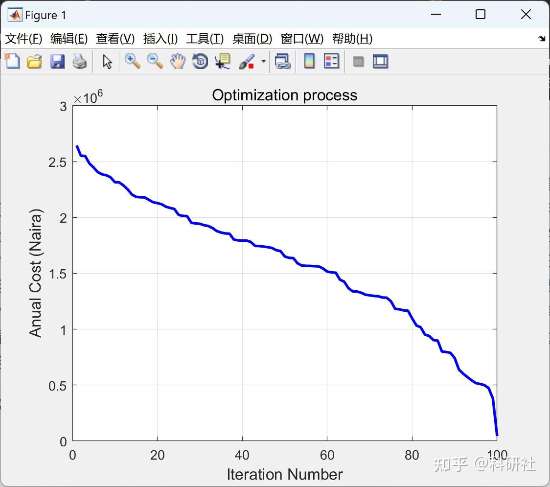
figure(1)
plot(Best_Object+Excess,'b','LineWidth',2)
grid on
title('Optimization process','fontsize',12)
xlabel('Iteration Number','fontsize',12);ylabel('Anual Cost (Naira)','fontsize',12);
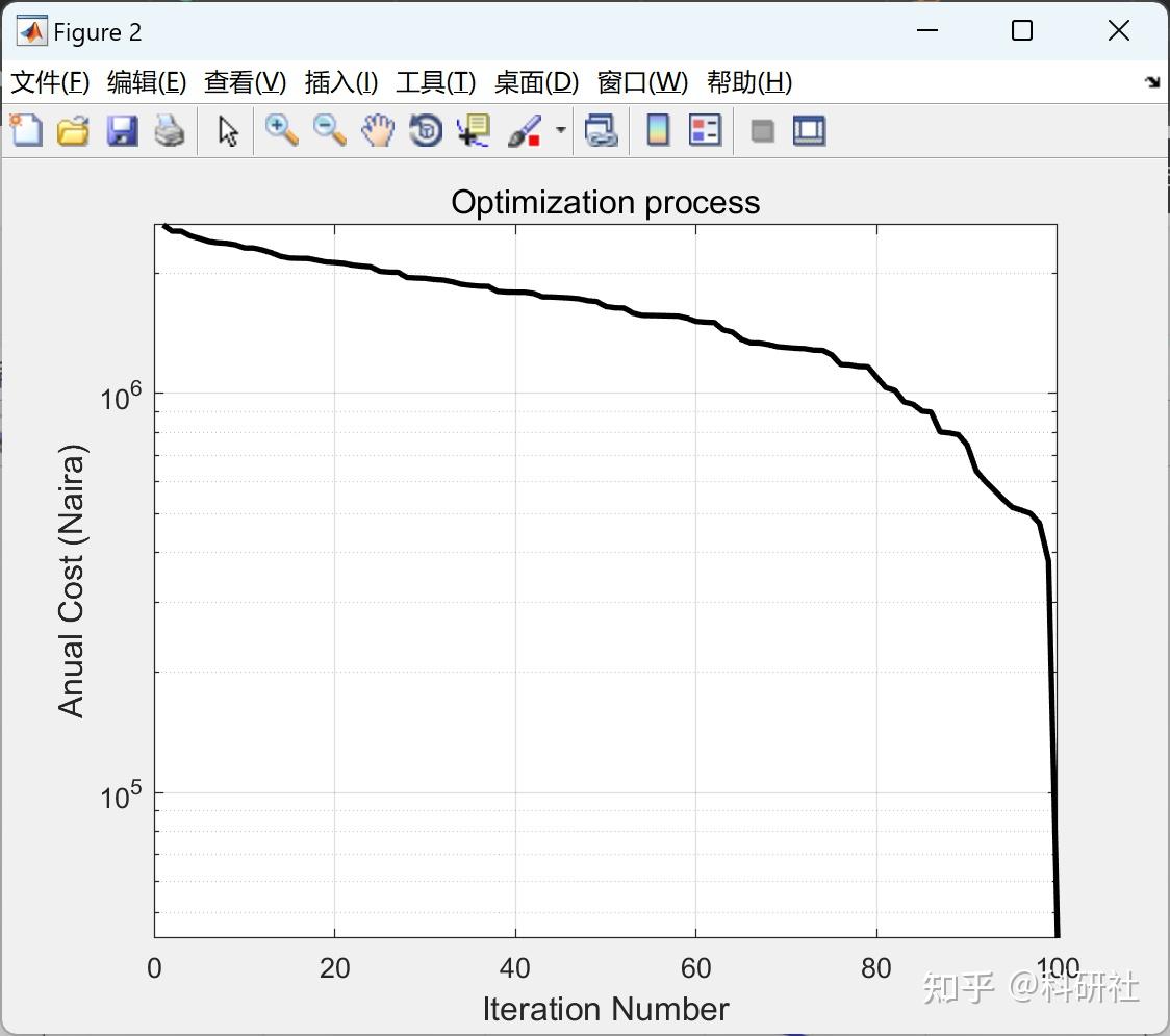
figure(2)
semilogy(Best_Object+Excess,'k','LineWidth',2);
grid on
title('Optimization process','fontsize',12)
xlabel('Iteration Number','fontsize',12);ylabel('Anual Cost (Naira)','fontsize',12);
% BestCost_Run=abs(BestCost_Run);
Best=Total_Cost
Worst=max(BestCost_Run+Excess)
Average=mean(BestCost_Run+Excess)
STD=std(BestCost_Run+Excess)
% figure('Name','Power Generated')
% bar(Power)
% xlabel('Time (Hours)')
% ylabel('Power (kW)')
% legend('PV Power','WT Power','Load','Battery Power')
文章中一些内容引自网络,会注明出处或引用为参考文献,难免有未尽之处,如有不妥,请随时联系删除。